This is a simple example of using the SML attenuation data for rainfall estimation.
The notebook is currently WIP...
import xarray as xr
import matplotlib.pyplot as plt
Load and plot example data from the OpenSat4Weather dataset
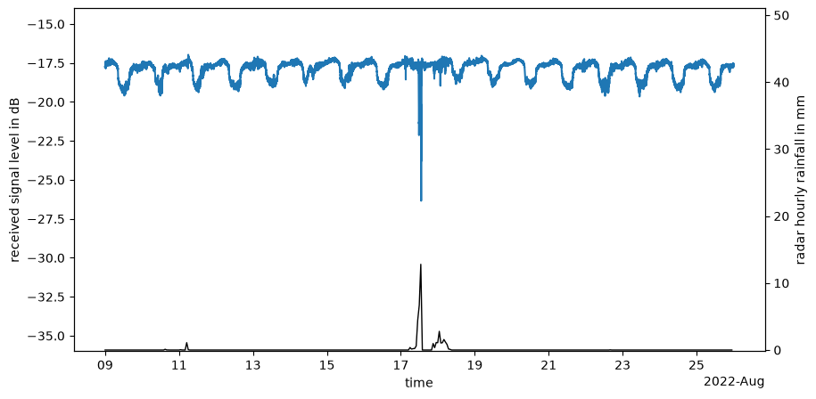
This is a short period of the OpenSat4Weather dataset (Nebuloni et al. (2025)) used for demonstration purposes.
ds_smls = xr.open_dataset('../misc/example_data/opensat4weather_example_sml.nc')
ds_radar_along_smls = xr.open_dataset('../misc/example_data/opensat4weather_example_radar.nc')ds_smlsLoading...
sml_id = 'FRA-00022'

fig, ax = plt.subplots(figsize=(10, 5))
ds_smls.rsl.sel(sml_id=sml_id).plot()
ax.set_ylim(-36, -14)
ax.set_ylabel("received signal level in dB")

ax2 = ax.twinx()
ds_radar_along_smls.rainfall_amount.sel(sml_id=sml_id).resample(time='1h').sum().plot(
    ax=ax2, color='k', zorder=-1, linewidth=1,
)
ax2.set_ylim(-0.2, 51)
ax2.set_ylabel("radar hourly rainfall in mm")
ax.set_title('')
ax2.set_title('')
ax.set_xlabel("time")
Use Kalman filters for wet-dry classification
This follows the approach described by Giannetti et al. (2018) based on code from the OpenSense training school https://
# The following functions were derived from the Kalman filter code from https://github.com/OpenSenseAction/training_school_opensene_2023

import numpy as np


def _kalman_filter(observations, Q, R):
    """Run a standard 1D Kalman filter on the given observations.

    NaN values in the observations are skipped: the state is carried
    forward unchanged for those time steps.

    Parameters
    ----------
    observations : array-like
        The measured signal to be filtered.
    Q : float
        Process variance.
    R : float
        Measurement variance.

    Returns
    -------
    xhat : np.ndarray
        The a posteriori state estimate (filtered signal).
    """
    z = np.asarray(observations, dtype=float)
    n_iter = len(z)
    sz = (n_iter,)  # size of array

    # allocate space for arrays
    xhat = np.zeros(sz)  # a posteri estimate of x
    P = np.zeros(sz)  # a posteri error estimate
    xhatminus = np.zeros(sz)  # a priori estimate of x
    Pminus = np.zeros(sz)  # a priori error estimate
    K = np.zeros(sz)  # gain or blending factor

    # intial guesses
    xhat[0] = np.nanmedian(z)
    P[0] = 1.0

    for k in range(1, n_iter):
        # time update
        xhatminus[k] = xhat[k - 1]
        Pminus[k] = P[k - 1] + Q

        # measurement update (skip NaN observations)
        if np.isnan(z[k]):
            xhat[k] = xhatminus[k]
            P[k] = Pminus[k]
            continue

        K[k] = Pminus[k] / (Pminus[k] + R)
        xhat[k] = xhatminus[k] + K[k] * (z[k] - xhatminus[k])
        P[k] = (1 - K[k]) * Pminus[k]
    return xhat


def Kalman_ST(rsl, Q=10e-5):
    R = 1  # estimate of measurement variance
    Q = 1e-3 # process variance
    return _kalman_filter(rsl, Q=Q, R=R)


def Kalman_FT(rsl):
    R = 1# estimate of measurement variance, change to see effect
    Q = 1e-1  # process variance
    return _kalman_filter(rsl, Q=Q, R=R)
sml_id = 'FRA-00022'
baseline_slow = Kalman_ST(ds_smls.rsl.sel(sml_id=sml_id).data)
baseline_fast = Kalman_FT(ds_smls.rsl.sel(sml_id=sml_id).data)
ds_smls.rsl.sel(sml_id=sml_id).plot(figsize=(10, 5))
plt.plot(ds_smls.sel(sml_id=sml_id).time, baseline_slow, label='baseline_slow', zorder=5)
plt.plot(ds_smls.sel(sml_id=sml_id).time, baseline_fast, label='baseline_fast')
plt.legend()
plt.xlim(ds_smls.time.sel(time=slice('2022-08-15', '2022-08-20')).min(), ds_smls.time.sel(time=slice('2022-08-15', '2022-08-20')).max())(np.float64(19219.0), np.float64(19224.999305555557))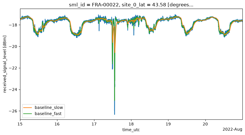
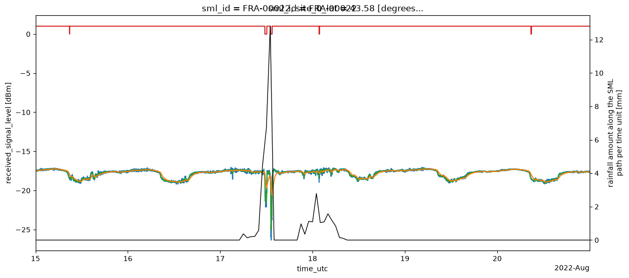
...WIP... wet-dry
fig, ax = plt.subplots(figsize=(14, 6))
ds_smls.rsl.sel(sml_id=sml_id).plot(ax=ax)
plt.plot(ds_smls.sel(sml_id=sml_id).time, baseline_slow, label='baseline_slow', zorder=5)
plt.plot(ds_smls.sel(sml_id=sml_id).time, baseline_fast, label='baseline_fast')
plt.plot(ds_smls.sel(sml_id=sml_id).time, (baseline_slow - 0.5) < baseline_fast, label='baseline_slow', zorder=5)
plt.xlim(ds_smls.time.sel(time=slice('2022-08-15', '2022-08-20')).min(), ds_smls.time.sel(time=slice('2022-08-15', '2022-08-20')).max())

ax2 = ax.twinx()
ds_radar_along_smls.rainfall_amount.sel(sml_id=sml_id).resample(time='1h').sum().plot(
    ax=ax2, color='k', zorder=-1, linewidth=1,
)
Calculate rain rate... WIP
- Nebuloni, R., Graf, M., Cazzaniga, G., Mercier, F., & Turko, M. (2025). The OpenSat4Weather dataset: Ku-band satellite link data for precipitation monitoring. 10.5194/essd-2025-537
- Giannetti, F., Moretti, M., Reggiannini, R., Petrolino, A., Bacci, G., Adirosi, E., Baldini, L., Facheris, L., Melani, S., & Ortolani, A. (2018). The Potential of Smartlnb Networks for Rainfall Estimation. 2018 IEEE Statistical Signal Processing Workshop (SSP), 120–124. 10.1109/ssp.2018.8450692